LTI Ratio | Interpretation |
|---|---|
< 1.0 | The building(s) are worth more than the land |
= 1.0 | Land and structures are valued equally |
> 1.0 | The land value is equal to or higher than the improvement value, redevelopment may be more likely |
4 Identifying Vacant and Potential Land for Redevelopment
Beyond the statutory requirements, identifying vacant and potentially redevelopable areas provides important context for this planning phase and supports analysis of the development potential of identified areas. These methodologies may serve as a starting point for identifying “commercially feasible” areas, as referenced in the statute. The inventory produced during this phase serves as a foundation for further study, not a final determination of development potential.
This section describes potential queries for identifying parcels within these categories, along with a set of analytical approaches that can be used to evaluate redevelopment potential. As with the rest of this guidance, these methods are offered as a flexible toolkit rather than a required methodology, allowing municipalities and COGs to recognize parcels that might support future housing development while tailoring the analysis to local priorities and conditions.
Regardless of the approach used, it is recommended that outputs be carefully reviewed using local knowledge, supplemental data sources, and/or aerial imagery.
For reference, the following datasets are used in the following analyses:
Parcel geometry: Connecticut CAMA and Parcel Layer (CT Housing Data Hub)
CAMA data: 2025 Connecticut Parcel and CAMA Data (CT Open Data Portal)
4.1 Vacant Parcels
Vacant parcels represent land that is either currently undeveloped or previously developed but now considered vacant. These parcels may present direct development opportunities. While no comprehensive statewide dataset of vacant parcels exists, the statewide CAMA and parcel dataset can be queried to identify parcels labeled as vacant.
Recommended query:
- State_Use for code “500”
- State_Use_Description for values such as “vac”, “vacant”, or “vacancy”
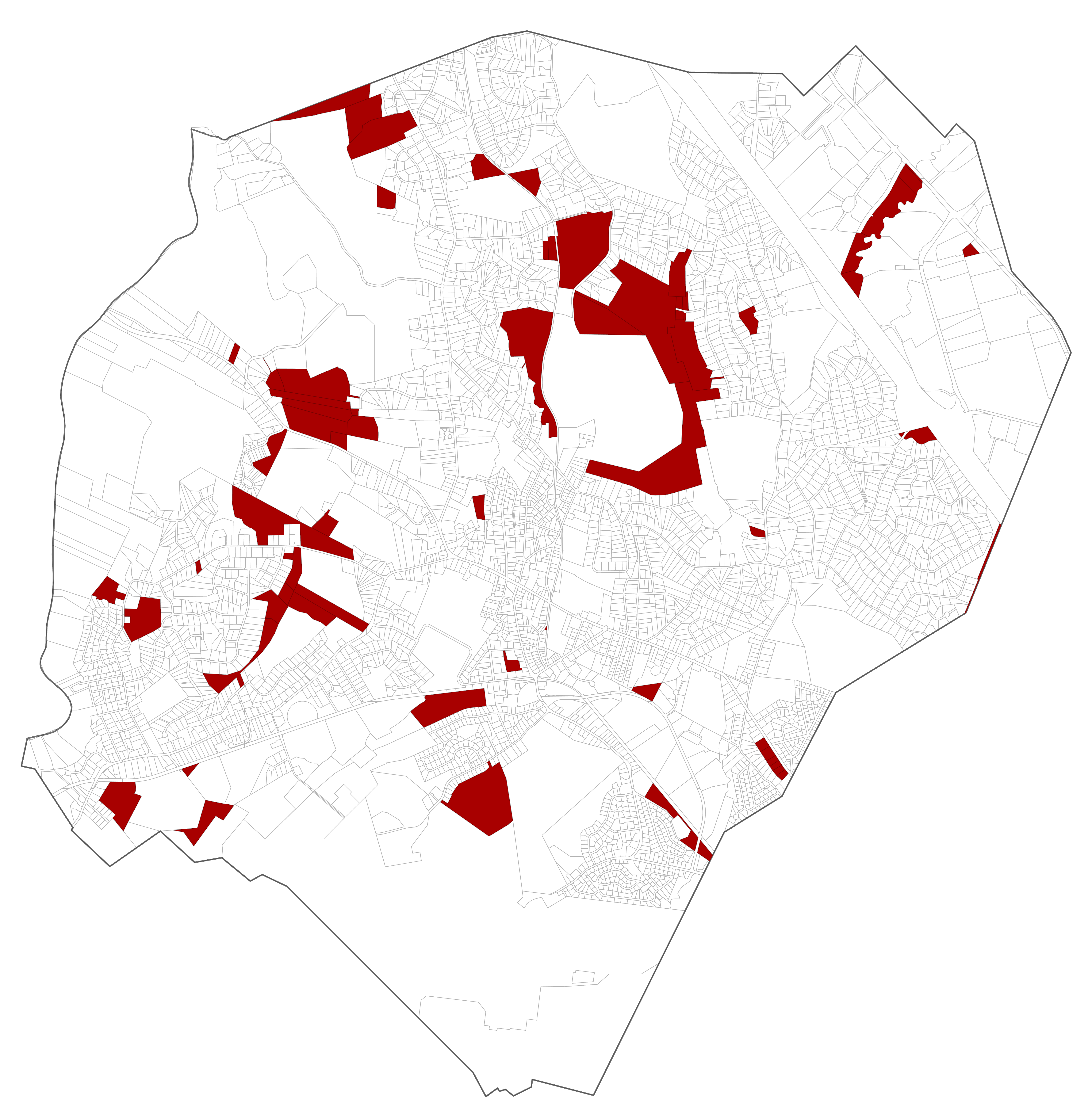
Example query logic:
STATE_USE IS '%500%'

OR STATE_USE_DESCRIPTION CONTAINS '%VAC%'4.2 Potentially Redevelopable Land
Potentially redevelopable land consists of previously developed parcels with characteristics suggesting they may be underutilized or suitable for redevelopment. The following approaches use data to systematically identify redevelopment opportunities; however, local knowledge and information are essential to confirm and verify results. These methods are not intended to be comprehensive, and other approaches may also be appropriate depending on local circumstances. Some approaches you might consider include the following:
Brownfields
Previously contaminated or industrial sites undergoing or eligible for cleanup.
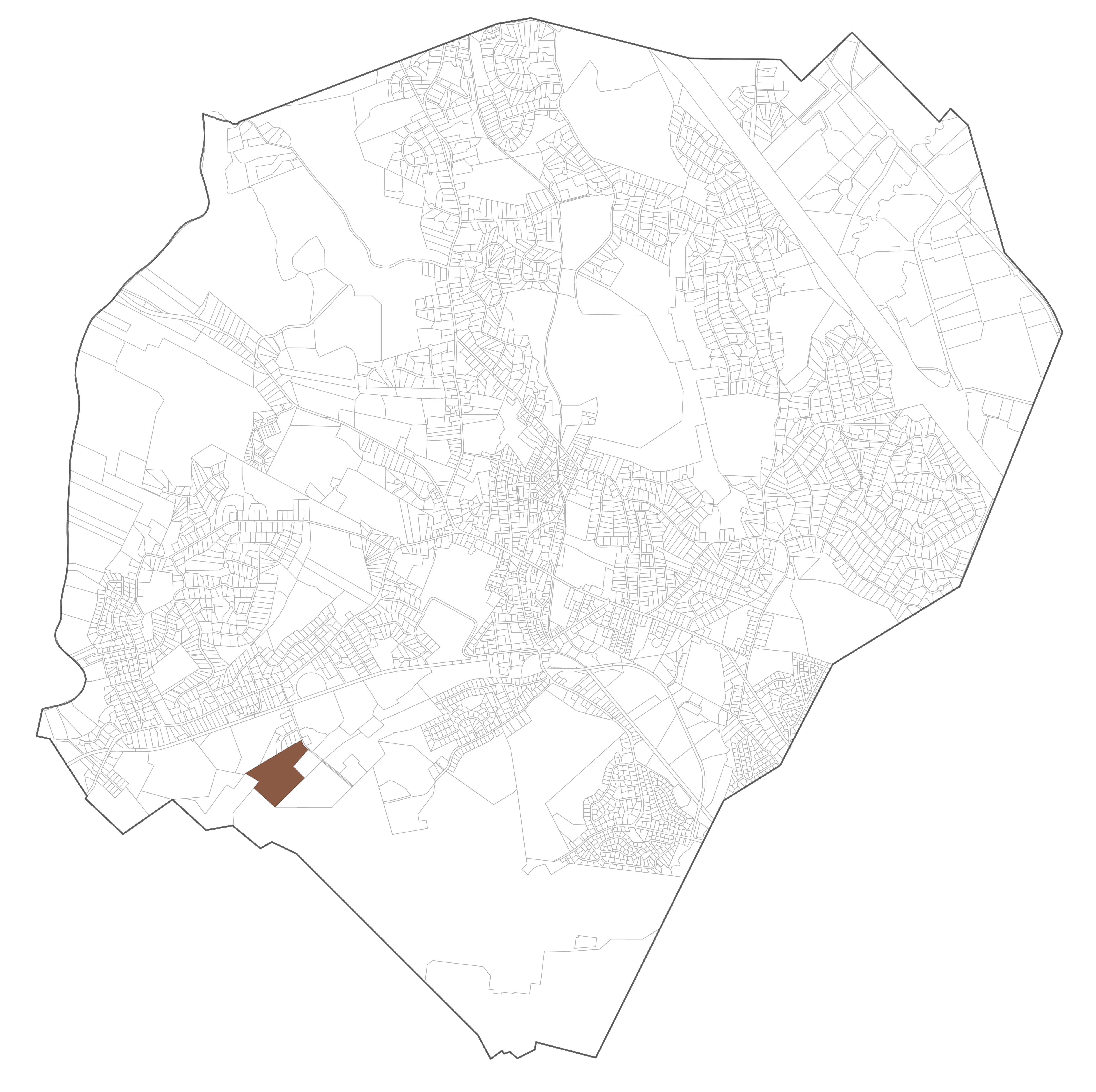
The available data describing brownfield site locations is provided by the Connecticut Department of Energy & Environmental Protection (CT DEEP). For more information, see the CT DEEP Connecticut Brownfields Inventory web page. This web page provides the locations in a tabular format in a .xlsx file. In addition the data is available as a geospatial layer as points, linked below.
Dataset: Brownfields
Inclusion of a brownfield site in the inventory does not automatically indicate that the site is feasible for redevelopment. Brownfield sites often require detailed environmental evaluation and may not be financially viable to remediate to residential standards, and some sites may have already been developed or remediated. Municipalities and COGs should carefully review brownfield sites using local knowledge and supplemental data before including them as potentially redevelopable, and should be mindful of environmental justice considerations.
Spatializing the data: If using the data in a tabular (.xlsx) format, it is necessary to spatialize it before processing with further analysis. If using the geospatial points layer, this step can be skipped. While geocoding to the address is feasible, it is recommended to use the Latitude and Longitude fields to create points corresponding to each brownfield site. The CRS should be NAD 83 Connecticut State Plane (2011). The following resources provide details on translating the tabular latitude and longitude data into geospatial points:
- ArcGIS Pro: XY Table to Point
- QGIS: Create Point Layer from Table
Identifying brownfield parcels: Use the points to identify the parcel geometry of the brownfield sites. This may be achieved with various queries, summary tools, or join tools that utilize spatial overlap. The following resources provide details and options for this process:
- ArcGIS Pro: Select by Location, Spatial Join, Summarize Within
- QGIS: Extract by Location or Select by Location within Vector Selection, Join Attributes by Location
Land-to-improvement value ratio
Analyze assessed land value to assessed improvements value in certain areas or districts to identify properties that may be underperforming (higher than average land-to-improvements values)
Calculating improvement values:
A land-to-improvement (LTI) ratio compares a parcel’s appraised building value to the value of that parcel’s land area. Parcels with exceptionally high LTI ratios have potential for redevelopment with higher-performing structures.
Improvement value can be found by totaling the combined appraised value of primary buildings, outbuildings (such as sheds and detached garages), and extra features (such as decks and patios). In the Connecticut CAMA and Parcel Layer, improvement values can be calculated by summing the “Appraised Building”, “Appraised Outbuilding”, and “Appraised Extra Feature” fields. The “Appraised Total” field should not be used in this analysis, as this field represents the combined appraised value of improvements and land.
Improvement = Appraised_Building + Appraised_Outbuilding + Appraised_Extra_Feature
Calculating LTI Ratios
After finding the total improvement value of each parcel, a new field of land-to-improvement ratios can be calculated. Divide the “Appraised Land” field by the newly created improvement field.
LTI_Ratio = Appraised_Land / Improvement
Interpreting the LTI Ratio
Because land and improvement values vary significantly across markets, any LTI threshold used to identify underperforming parcels should be based on local market conditions and development patterns.
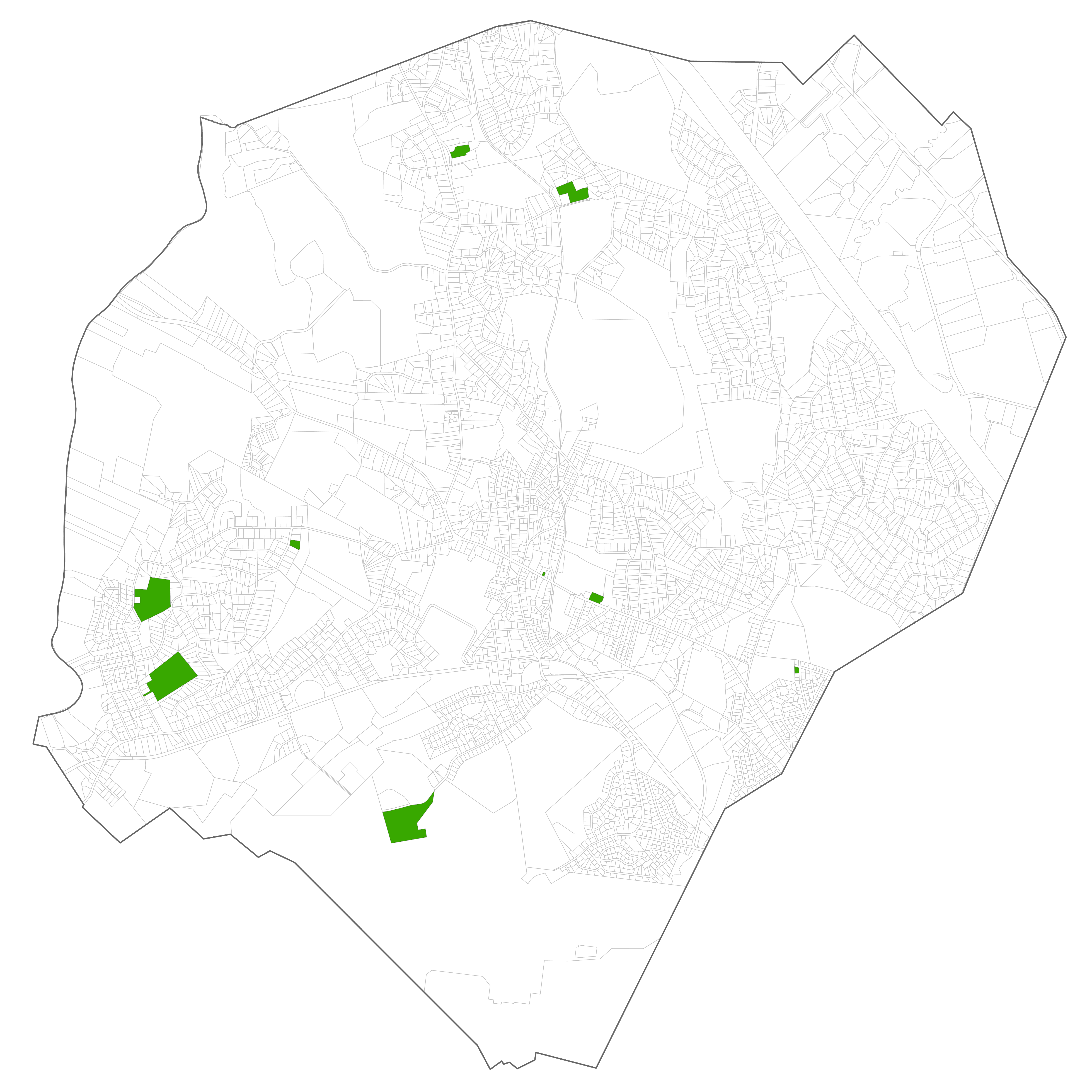
Parcel size relative to district average
Analyze parcel size by neighborhood or regulatory district to identify parcels that may be underutilized (significantly larger than the average) which may indicate an opportunity for infill development
The feasibility of redevelopment efforts is also dependent on parcel size; accordingly, potentially redevelopable land analyses may include an inventory of parcels with the largest relative area within their neighborhood designation.
The “Land Acres” field in the Connecticut CAMA and Parcel Layer may have missing or incomplete data so it is recommended to use the “Shape Area” field or to derive acreage directly from the parcel geometry in GIS.
Normalizing parcel area by neighborhood
To identify parcels that are larger than others in their neighborhood, an analyst should select a threshold, such as the top 10% of parcel area within each neighborhood or district, to flag potential infill opportunities.
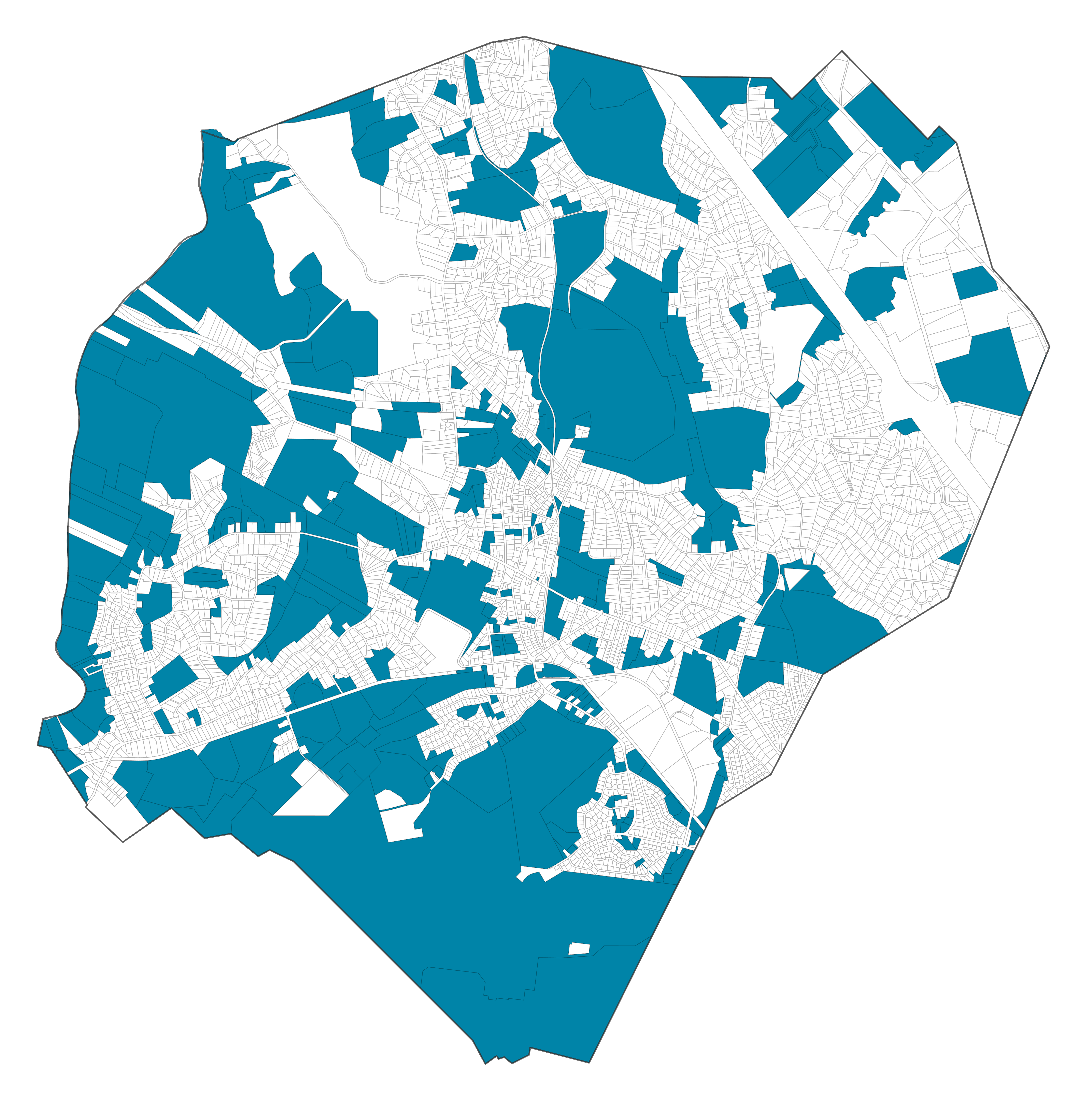
Floor Area Ratio (FAR) analysis
Analyze Floor Area Ratios by neighborhood or district to identify parcels that have significantly lower than average ratios which may indicate infill or redevelopment opportunities
The floor area ratio (FAR) of a parcel’s primary building is the ratio of gross building area to lot or parcel area. Higher FAR values indicate higher building density, and lower potential for redevelopment. Whereas land-to-improvement ratio measures the economic value of existing buildings, the floor area ratio measures the physical space a building occupies, weighted by number of floors.
The Connecticut CAMA and Parcel Layer field “Gross Area of Primary Building” represents the sum of all enclosed living and non-living building spaces. The gross building area is measured from a building’s exterior and factors in number of floors, extending beyond the building footprint.
In some cases, the “Gross Area of Primary Building” field may have missing or incomplete data, in which case the “Living Area” field may be used as a substitute. Note that this is a more restrictive metric, as it only captures habitable, finished floor space rather than total enclosed building area.
Calculating the FAR
A new field of FAR values can be calculated by dividing the “Gross Area of Primary Building” field by the parcel area field, such as the “Shape Area” field in the Connecticut CAMA and Parcel Layer.
FAR = Gross Floor Area / Total Lot Area
As previously stated, the “Shape Area” field or a parcel geometry area calculation should be used over the “Land Acres” field, as the latter may have missing or incomplete data.
Interpreting the FAR
Unlike land-to-improvement ratios and relative parcel size, floor area ratio and potential for redevelopment have a negative relationship: higher FAR values indicate less possibility for redevelopment.
To identify underperforming parcels using FAR, select a threshold at the lower end of the distribution as these represent properties where the built floor area is small relative to the land area, suggesting potential for more intensive development.
FAR Ratio | Interpretation |
|---|---|
< 1.0 | The building's total square footage is smaller than the lot. This indicates low-density development, such as single-family homes or suburban subdivisions. |
= 1.0 | The total building size is exactly equal to the lot size. This means you could build a one-story building covering the entire lot, or a two-story building covering half the lot. |
> 1.0 | The building space exceeds the lot size, indicating multi-story, high-density development. For example, a 10-story building occupying 10% of a lot yields a high FAR. |
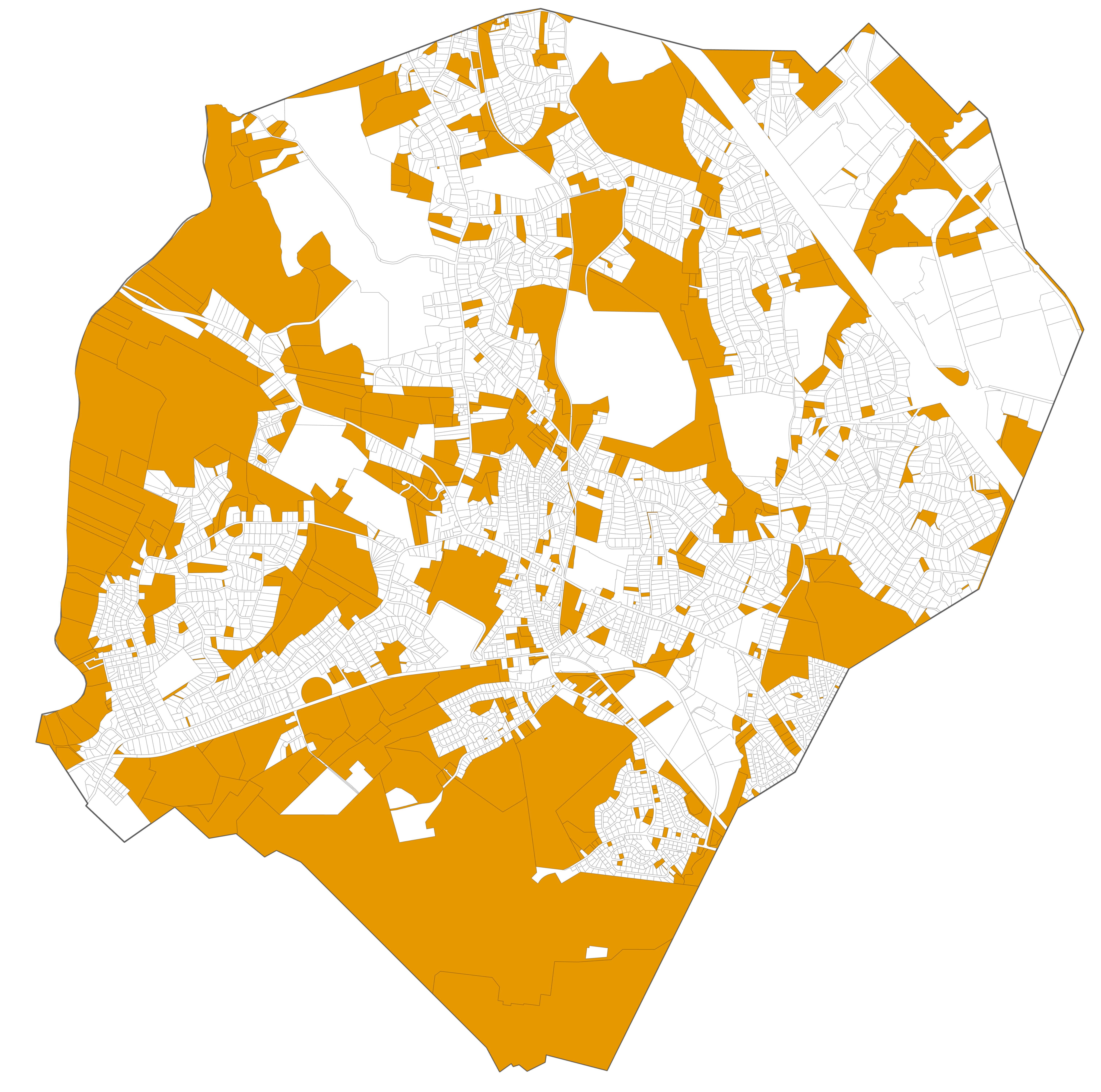
Construction and renovation year clustering
Analyze construction and renovation years to identify clusters of existing units in need of rehabilitation.
Construction and renovation year clustering offers insight into building aging patterns within municipalities, with the goal of identifying parcel clusters that may need rehabilitation.
The Connecticut CAMA and Parcel Layer has multiple fields relevant to this analysis.
- “AYB” (Actual Year Built) field: The original construction date for each parcel’s primary building
- “EYB” (Effective Year Built) field: The building’s effective age, factoring in remodeling and renovations.
- “Condition Description” field: Ordinal, categorical data indicating the physical condition of a building.
It is important to note that there are no statewide criteria for evaluating Effective Year Built. The calculation of effective building age may vary depending on the individual judgement of assessors and is a form of subjective data. Accordingly, if the AYB and EYB fields lack sufficient data or if municipalities have their own criteria for evaluating EYB, they may elect to use their own assessor data and property records.
Construction and renovation year clustering analysis
This analysis uses a multivariate clustering tool to group parcels based on three fields simultaneously: original construction date (AYB), effective building age (EYB), and physical deterioration (Condition Description). Rather than applying a single threshold to one variable, multivariate clustering evaluates all three fields at once, automatically grouping parcels based on combinations of age, renovation history, and physical condition. The result is multiple groups of parcels, one of which will represent aged, infrequently renovated, and deteriorated buildings within the study area, which are the parcels most likely to be candidates for rehabilitation or redevelopment.
Why multivariate clustering?
A simple threshold approach (for example, filtering only by construction year) would miss properties that are old but have been well-maintained, or flag properties that are deteriorated but have been recently renovated. A multivariate analysis using the “AYB”, “EYB”, and “Condition Description” fields together can be used to flag groups of parcels with high redevelopment potential.
It is important to avoid clustering methods that rely on spatial relationships between parcels, including proximity or adjacency. Spatial clustering methods, such as K-nearest neighbor (KNN) algorithms or techniques informed by Queen contiguity, would traditionally be used for parcel data using polygon geometry. These identify parcels based on how close they are to each other or whether they share edges or corners. Because the parcel layer may be segmented by missing data, these methods will fail or produce inaccurate clusters by attempting to connect parcels across large gaps. In contrast, a non-spatial multivariate clustering method ensures that all parcels with available data are assigned to a cluster with shared features, regardless of where they are located. For more insight into spatial methods and their limitations:
- Brief introduction to concepts, with R examples: Spatial Weights Matrix
- Description of spatial statistics: Modeling Spatial Relationships
- Overview of ESRI clustering tools and their applications: Mapping Clusters
Therefore, it is recommended to use a solely trait-based multivariate clustering tool. These tools identify optimized seed locations, around which clusters will be built, by maximizing their initial distance from each other. The tool then repeatedly adjusts these seeds to minimize trait variability within clusters and maximize trait variability between clusters. In this way, all parcels with available data are assigned to a cluster with shared features. Simplified, the process is:
assign seeds → recompute and adjust seed location → repeat until stable
The following tools and settings are recommended for conducting this analysis in GIS software:
- ArcGIS Pro: Multivariate Clustering
- QGIS: Attribute Based Clustering Plugin
Recommended settings:
- K-means algorithm
- Optimized seeds
For the ArcGIS Pro tool, there is an option to choose between the K-means or K-medoids algorithm. K-medoids is robust to outliers, while K-means is faster and operates more efficiently with large datasets; accordingly, K-means is the recommended algorithm for this analysis and is also the default option for the QGIS Attribute Based Clustering Plugin.
Within these tools, municipalities must also choose the number of clusters to evaluate. Considerations when choosing number of clusters (K) include:
- Additional statistical measures (pseudo-F statistic)
- Interpretability
- Validation against imagery layers
- Local knowledge
The chart below is a built-in product of the Multivariate Clustering Tool in ArcGIS Pro. The local peaks indicate a higher pseudo-F statistic, corresponding to greater distinctiveness between clusters and more meaningful data separation.
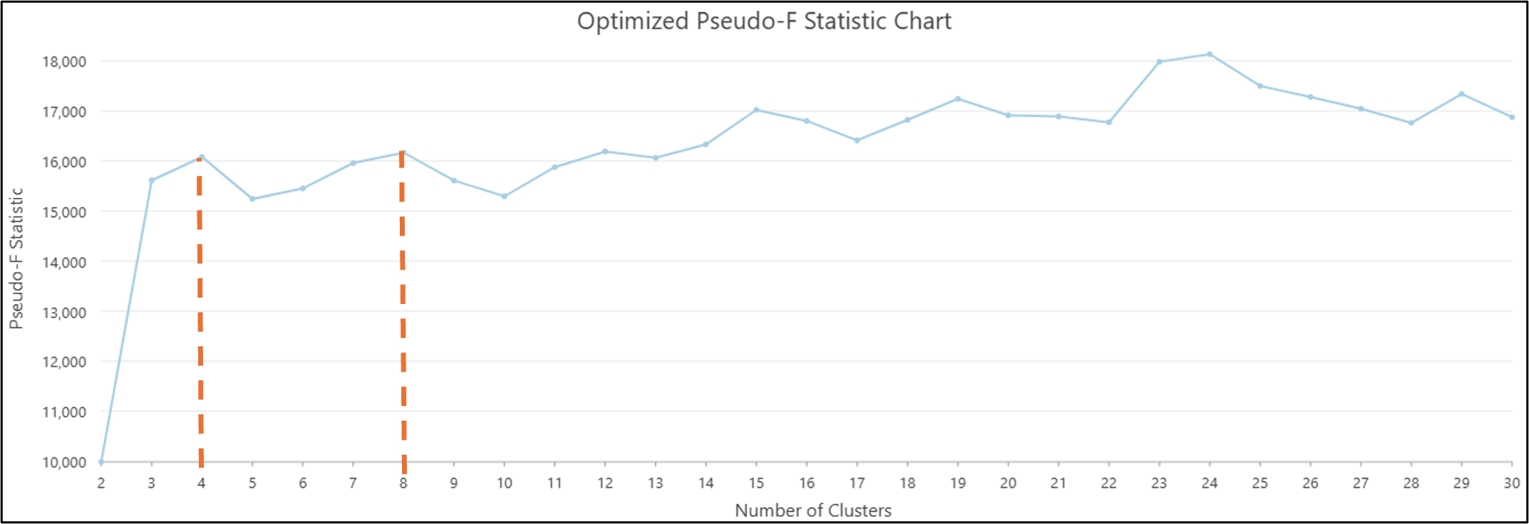
Based solely on the chart, the most appropriate number of clusters would be 4 or 8. In general, a larger number of clusters means that a smaller, more selective subset of parcels will be identified. While 8 clusters may offer a more refined analysis and statistically stronger results, 4 clusters offer simplicity and ease of interpretation.
For construction and renovation year clustering analyses, it is generally recommended to evaluate results from 3 to 6 clusters. This range should be sufficient to capture meaningful variations in housing characteristics while maintaining interpretability. Therefore, the selection of appropriate number of clusters (K) does not have to rely solely on statistical measures but also on the practicality of the resulting groups. In addition to these considerations, it is important to check whether the redevelopment candidates make sense when mapped and validated against other data such as imagery.
The multivariate analysis may need to be run multiple times to settle on the most suitable number of clusters. When evaluating analysis outputs, it is important to verify whether each cluster represents a distinct and understandable housing profile based on the three fields of interest.
Data preparation
Prior to running a multivariate clustering analysis, municipalities should translate the categorical Condition Description field into a new field of quantitative data, with buildings in poorer condition receiving lower numerical scores. Municipalities may need to evaluate Condition Description data in the context of their individual assessing standards to accurately translate them to numbers, as there are no statewide standards for this field. Additionally, the data may need to be cleaned by removing inconsistent capitalization, spelling, or spacing prior to creating a new field.
Example numerical classification dictionary:
- “Very Poor”: 1
- “Poor”: 2 ”
- Average-“: 3
- “Average”: 4
- “Average+”: 5
- “Good”: 6
- “Very Good”: 7
- “Excellent”: 8
If the multivariate clustering tool in a municipality’s software of choice does not automatically standardize data, it is necessary to standardize the EYB, AYB, and numerically transformed Condition Description fields due to scale differences.
Within the Connecticut CAMA and Parcel Layer, the AYB and EYB fields may include null placeholder values in the form of extremely low or high numbers. Accordingly, municipalities should evaluate the distribution of these values in their CAMA data, identify any outliers or apparent null placeholders, verify these against their oldest historical buildings, and filter this data out prior to running the clustering analysis.
Within the Connecticut CAMA and Parcel Layer, the AYB and EYB fields may include null placeholder values of 0, 15, or other extremely low numbers. Placeholders may also take the form of years from the 1500s, 1600s, or 1700s. Accordingly, municipalities should evaluate the distribution of AYB values in their CAMA data, identify any outliers or apparent null placeholders, verify these against their oldest historical buildings, and filter this data out prior to running the clustering analysis.
Example filter queries include:
- “EYB” is not equal to 0
- “EYB” is less than or equal to 2025
- “AYB” is greater than or equal to 1639 (the construction year of the Henry Whitfield House, the oldest standing building in Connecticut)
- “AYB” >= 1788 (the year of Connecticut’s founding as a state)
- “AYB” >= 1899 (a common placeholder year, as it is the zero date in systems like SQL, Power BI, and SharePoint)
Interpreting results
Below is a sample series of boxplots automatically produced by running the Multivariate Clustering tool in ArcGIS Pro. These boxplots illustrate the distribution of data for the three fields of interest, as well as which clusters contain the combination of traits most relevant to this analysis.
The red line, indicating cluster 2, reveals the target relationship. Cluster 2 contains the lowest values of EYB and numerically transformed Condition Description, as well as values of AYB below the median. In this case, the parcels in cluster 2 would be isolated and included in a Potentially Redevelopable Land inventory.
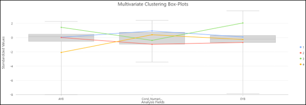
Note that AYB will naturally contain lower values than EYB, as it reflects original construction rather than effective age. Additionally, the oldest buildings may have already undergone extensive renovation and may not exhibit similarly low condition ratings or EYB. Therefore, the numerically transformed Condition Description and EYB fields should be weighted more heavily than AYB when deciding which cluster to isolate, as these variables better reflect the current redevelopment potential of properties.
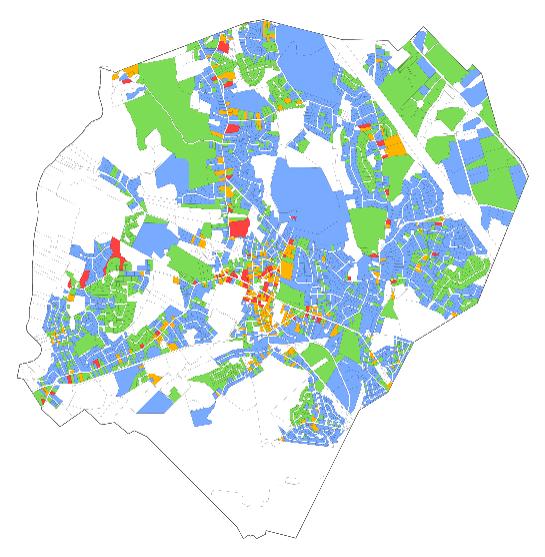
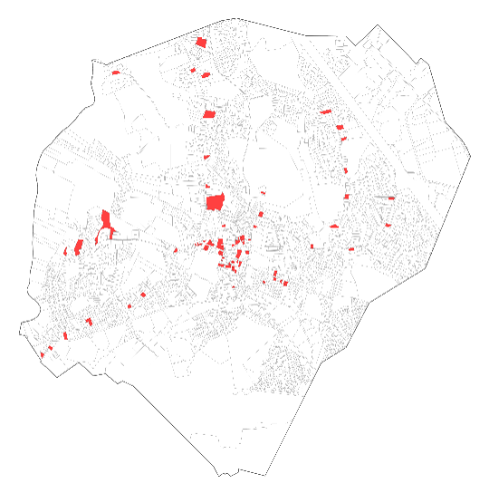
The figure on the left shows the results of the Multivariate Clustering tool in ArcGIS Pro, where cluster colors on the map correspond to those shown in the boxplots. The figure on the right shows the resulting map after isolating cluster 2, which represents the end product of a construction and renovation year clustering analysis.